
May 17, 2024
Updated July 30, 2024
Guidance on curve-fitting techniques related to measurements associated with nerve stimulation compliance
This notice provides further guidelines on curve-fitting techniques being used in accordance with section 5.3.1 of RSS-102.NS.MEAS or 7.1.1 of SPR-002.
Until instructed otherwise, when submitting an enquiry for approval of the curve-fitting technique, the analysis should include the following:
-
A description of the Equipment Under Test (EUT);
-
The maximum field strength (MFS) values for both the magnetic (H) and electric (E)-fields;
-
The measurements grid to identify the MFS, including the description of the plane where the analysis is conducted (XY, XZ and YZ);
- All observations are made perpendicular to the plane of evaluation
-
The number of samples and the spatial resolution used during the test;
- A minimum of 10 samples (measurement points) are required.
- While the vast majority of the samples should be measured where 𝑑meas ≥ 1.7𝐷p (Equation 1 in RSS-102.NS.MEAS) is met, it is permitted to measure some samples closer.
- Include the models (linear and/or non-linear) and their empirical functions;
- A minimum of 3 models are required.
- For polynomial regression models, the order of the model shall be increased until signs of overfitting become evident.
Note: Overfitting may occur when the model is too complex. In an overfitting situation, adjusted 𝑅2 does not increase or starts to decrease as higher order of polynomial are added to the regression model.
- Analytical methods can confirm your results. Ampere's law for H-fields can be included as an option.
- Include a comparison table with the values of the Multiple 𝑅, 𝑅2, adjusted 𝑅2, Standard error of the regression (S), number of samples and estimated values at touch position (0 mm);
- The applicant must use a confidence level of 95% or higher in all models presented in the comparison table.
- The applicant is responsible to use the model with the lowest S.
Notwithstanding the above conditions, ISED may request an analysis with a higher confidence level or a smaller regression error if deemed necessary.
An example of an acceptable curve-fitting analysis using the Biot-Savart law can be found in the Annex.
Annex – Curve-fitting analysis Example
Objective: Predict the value of the H-Field at touch position
Four basic steps are needed to conduct a proper curve-fitting analysis as listed below and illustrated in Figure 1:
1. Locating the Maximum Field Strength (MFS),
2. Data Collecting Process,
3. Performing Curve-fitting, and
4. Analyzing the Results.
Figure 1: Overview of the curve-fitting analysis

Step 1 – Locating the MFS
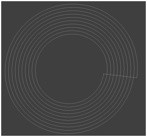
In this example, our EUT will be a coil with the following parameters (see Figure 2)
-
Outer radius: 40 mm
-
Inner radius: 20 mm
-
Number of turns: 10
-
Current: 1 A rms
-
Frequency: 370 kHz
Figure 2: EUT being used in the example
Methodology:
-
Start gathering the data
-
Measurements are made perpendicular to the XY plane
-
Locate the MFS in the XY plane
Do not assume the center of a coil will yield the MFS
Figure 3: Grid for the evaluation of the MFS
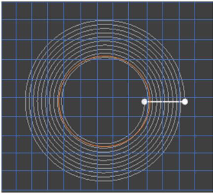
- A grid of 20mm by 20mm as shown in Figure 3 was selected in this example. (Note that the spatial resolution will depend on the size of the EUT and the probe).
- A probe is used to measure the E- and H- fields stemming from the EUT. (For simplicity, this example will only explore the H-field).
- These initial measurements are made at Z = 3.5 mm from the surface of the XY plane.
- The MFS of the magnetic field is located at 20 mm from the center of the coil (237.72 A/m)
The resulting magnetic H-field strength was plotted against the distance in Figure 7.
Figure 4: Measured H-field in relation to distance
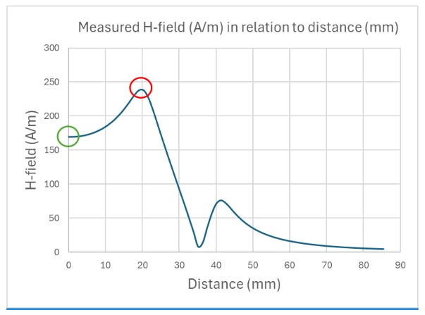
- The maximum H-field strength (237.72 A/m) on this plot occurs at 20 mm from the center of the coil (see red circle).
- Note that the center of the coil did not yield the maximum H-field strength. The center of the coil was measured to have an H-field of 169.53 A/m (see green circle).
-
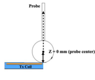
The probe must therefore be placed at 20 mm from the center of the coil to gather electric or magnetic values when measuring along the Z-axis. (see Figure 5 below).
Figure 5: Probe located in the MFS location
Step 2 – Data Collecting Process
Once the MFS is located, we proceed to collect the 11 measurement points that will be used to build the predictive model. In this example we measured 11 data points at varying distances (z-direction) from the coil. The resulting data is captured in Table 1.
| Distance (mm) | H-Field (A/m) |
| 3.5 | 237.72 |
| 5.4 | 196.99 |
| 7.5 | 163.58 |
| 10.0 | 134.85 |
| 12.9 | 109.80 |
| 16.4 | 87.98 |
| 20.5 | 69.16 |
| 25.4 | 53.18 |
| 31.2 | 39.87 |
| 38.2 | 29.05 |
| 46.0 | 20.89 |
Step 3 – Performing Curve-fitting
In this example, we use six (6) regression techniques to validate their model errors.
- Model 1: Linear Regression
- Model 2: Quadratic Regression
- Model 3: Cubic Regression
- Model 4: 5th Order Regression
- Model 5: 7th Order Regression
- Model 6: 8th Order Regression
To be concise, the 4th and 6th order are not shown in this example.
Each regression model will use the 11 data points from Table 1. In this example, the Data Analysis package included in MS Excel was used to perform the regression analyses.
Important: When submitting information to ISED, the applicant must provide their own equations. The models in this guidance are merely used to illustrate the process.
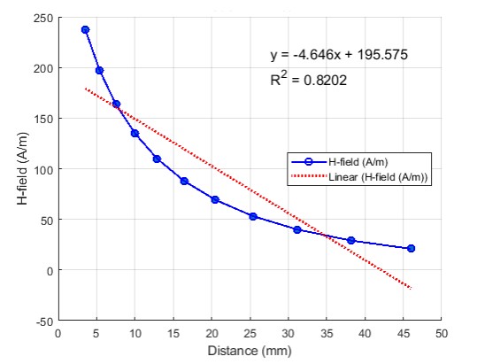
Model 1: Linear Regression
Figure 6: Model 1 - Linear regression
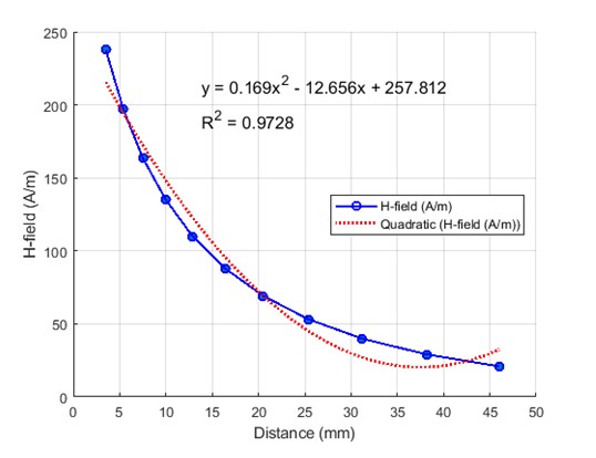
Model 2: Quadratic Regression
Figure 7: Model 2 - Quadratic regression
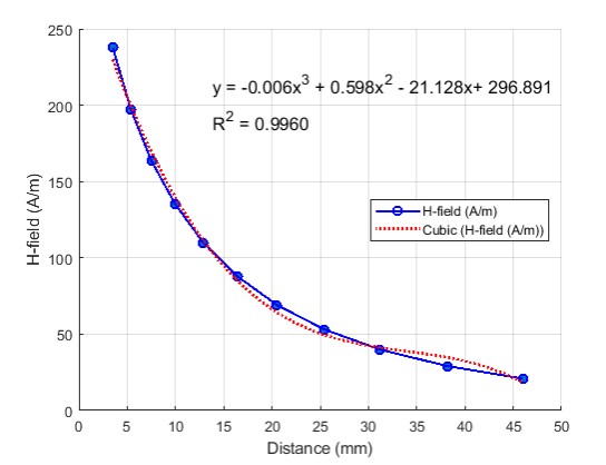
Model 3: Cubic Regression
Figure 8: Model 3 - Cubic Regression
Model 4: 5th Order Regression
Figure 9: Model 4 - 5th Order Regression

Model 5: 7th Order Regression
Figure 10: Model 5 - 7th Order Regression

Model 6: 8th Order Regression
Figure 11: Model 6 - 8th Order Regression

Step 4 – Analyzing Results
After completing the 6 regression models, we compared the output of each model. The data shown below is directly obtained from use of the models built into Microsoft Excel. Users are free to use the software package they’d like. The results are shown in Table 2 below:
|
Parameter |
Linear Regression Model | Quadratic Regression Model | Cubic Regression Model | 5th Order Regression Model | 7th Order Regression Model | 8th Order Regression Model |
|---|---|---|---|---|---|---|
| Multiple R | 0.906 | 0.986 | 0.998 | 1.000 | 1.000 | 1.000 |
| R2 | 0.820 | 0.972 | 0.996 | 1.000 | 1.000 | 1.000 |
| Adjusted R2 | 0.800 | 0.966 | 0.994 | 1.000 | 1.000 | 1.000 |
| Standard Error (S)* | 32.153 | 13.269 | 5.452 | 0.848 | 0.157 | 0.186 |
| Number of data points used | 11 | 11 | 11 | 11 | 11 | 11 |
| Estimated magnetic field strength at touch position (A/m) | 195.575 | 257.812 | 296.891 | 338.757 | 356.491 | 358.419 |
* The units of the standard error are the units of the measured variable A/m in this example.
As shown in Table 2, the 7th order regression model produced the lowest standard error. From the model, the estimated magnetic field strength at touch position 356.491 A/m, and the predicted lower and upper bounds are 349.330 to 363.652 A/m respectively. The regression analysis utilized a confidence level of 95%, which is the minimum value that should be used by applicants. While this example illustrates a product which would be non-compliant (with the limit in this case being 90 A/m), it nonetheless demonstrates the necessary steps for curve-fitting, to establish compliance in real-world situations. Note that the 8th order regression model was not selected as evidence of overfit were shown by the increase of S.